Large Language Models (LLMs) are rapidly becoming part of everyday life. As these systems interact with users, an important question emerges:

Which responses do people actually prefer?

In this Kaggle competition, each sample contains a prompt and two responses generated by anonymous chatbots. Human annotators select the response they prefer: Model A, Model B, or a tie. The challenge is to build a model that can predict these preferences.

This was my first Kaggle competition. Because the competition runs indefinitely and has no prize pool, it provided a low-stakes environment to experiment and learn.

After several iterations, my final model achieved a log-loss score of 1.02, placing 36th out of 213 submissions at the time of writing.

Competition link: https://www.kaggle.com/competitions/llm-classification-finetuning

Code: https://www.kaggle.com/code/danman1432/llm-classification-finetuning

Data Preparation and Feature Engineering

Problem Setup

The goal of the competition was to predict which of two chatbot responses a user would prefer for a given prompt. Each example contains:

• a prompt
• response A
• response B
• the human preference:
  • Model A wins
  • Model B wins
  • Tie

This makes the problem a three-class classification task.

Dataset Overview

The competition provided three files:

Training dataset

Contains the prompt. both model responses, and labels indication whether the user preferred Model A, Model B, or tie.

Test dataset

Has the same structured as training data but without preference labels. The goal is to predict probabilities for each possible outcome.

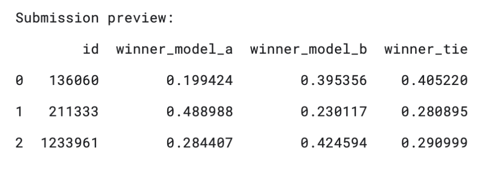
Sample submission

Shows the required format for predictions, with probabilities for winner_model_a, winner_model_b, winner_tie.

Feature Engineering

The raw dataset contains mostly text which has to be converted into features that a model could learn from.

Target Variable

The original dataset included three indicator columns representing the winning response. These were converted into a single multi-class target variable:

• 0 -> Model A wins
• 1 -> Model B wins
• 2 -> Tie

This simplifies the task into a standard three-class classification problem.

Structural Features

Before working with the text itself, I created numerical features describing the structure of the responses.

Length-based features

• Word count
• Character count
• Sentence count
• Difference in word count
• Difference in character count
• Ratio of response lengths

These features help capture situations where one model tends to produce longer, more detailed answers, while the other produces shorter or more concise responses.

Stylistic Features

I also added simple indicators of writing style:

• Average word length
• Number of exclamation points
• Number of question marks
• Number of line breaks

These features capture stylistic differences such as formatting, rhetorical questions, or expressive language.

Prompt alignment features

Another useful signal is how closely each response relates to the original prompt. To measure this, I computed:

• Prompt overlap with response A
• Prompt overlap with response B
• The difference between the two

This helps the model detect when one response is more aligned with the question being asked.

Constructing the Final Text Fields

Finally, each response was paired with the original prompt to create two combined text fields:

• pair_a: prompt + response A
• pair_b: prompt + response B

This allows later stages of the pipeline to evaluate each response in the context of the question it is answering, rather than analyzing the response in isolation.

Converting Text into Features with TF-IDF

Next step was to transform raw text into numerical features that a machine learning model could use. Because the dataset consists of prompts and two competing responses, the challenge is comparing two pieces of text relative to the same response.

Why TF-IDF?

Machine learning models cannot work directly with raw text, so the responses first need to be converted into numerical features. To do this, I used TF-IDF. TF-IDF assigns higher weights to words that are important in a specific document but relatively rare across the entire dataset. Words that appear everywhere (like “the” or “is”) receive lower weights. This helps highlights informative terms rather than common filler words. Because each response was already paired with its prompt (pair_a and pair_b), the TF-IDF representation allows the model to learn relationships between the instruction and the generated answer.

Capturing Phrases with N-grams

Single words sometime miss important context. For example, the phrase “not allowed” carries a different meaning than the individual words “not” and “allowed”. To capture these patterns, I used n-grams, which represent sequences of words.

• Unigrams (1-grams) – individual words
• Bigrams (2-grams) – two word combinations

For example, the sentence:

“The capital of Japan is Tokyo”

would produce

Unigrams:

• “The”
• “capital”
• “of”
• “Japan”
• “is”
• “Tokyo”

Bigrams:

• “The capital”
• “capital of”
• “of Japan”
• “Japan is”
• “is Tokyo”

Including bigrams allows the model to capture short phrases and local context, which can be important when comparing responses.

Limiting the Vocabulary Size

Using bigrams dramatically increases the number of possible features. To keep the model manageable, I limited the TF-IDF vocabulary to 30,000 features. Here, a feature refers to a word or phrase in the vocabulary. Each document is represented as a vector of length 30,000, where each position corresponds to the TF-IDF weight of a specific term. This keeps the representation expressive while preventing the feature space from blowing up.

Comparing the Two Responses

After generating TF-IDF vectors for both responses, I computed their difference. This difference vector highlights which words or phrases appear more strongly in one response than the other. This representation gives the model direct information about how the two answers differ, which is often more useful than analyzing them independently.

Summary of Text and Structural Features

All features were combined into a single dataset before training the model. These features included:

• TF-IDF features for response A
• TF-IDF features for response B
• TF-IDF difference vector (A-B)
• Engineered numerical features

Together, these features capture both semantic information from the text and structural signals from the responses.

Modeling, Training, and Evaluation

After transforming the dataset into numerical features, the next step was training a model capable of predicting whether Response A, Response B, or both responses would be preferred. For this task, I used LightGBM, a gradient boosting algorithm that works well with large, sparse feature spaces like those produced by TF-IDF.

Why LightGBM?

LightGBM was a good fit for this problem for several reasons:

• It performs well with high-dimensional sparse data
• It can handle mixed feature types (text features and numeric features) without additional scaling
• It captures non-linear relationships efficiently
• It trains quickly even on large datasets

Training Setup

To evaluate the model during development, I created an 80/20 train-validation split from the training dataset. Because gradient boosting models can easily overfit if allowed to train indefinitely, I used early stopping. Training stops when the validation loss stops improving for a specified number of iterations. This prevents the model from memorizing training data and identifies the optimal number of boosting rounds.

To further reduce overfitting, I applied several regularization techniques:

• leaf contraints
• feature subsampling
• L1 and L2 regularization penalties

Validation Results

On the 20% validation set, the model achieved:

• Log-loss: 1.019
• Accuracy: 48.8%
• Best iteration: 167 boosting rounds

For a three-class problem, random guessing would produce an accuracy of roughly 33%, so the model performs substantially better than chance. Although training was allowed to run up to 2000 boosting rounds, early stopping identified 167 as the optimal point. This suggests that most of the useful learning happened early in training.

Predicted Class Distribution

The model’s predictions were distributed as follows:

• Response A wins: 38.4%
• Response B wins: 36.2%
• Tie: 25.4%

This distribution is reasonably balanced and reflects the fact that many examples in the dataset involve clear preferences between the two responses.

Confusion Matrix Insights

Examining the confusion matrix reveals an interesting pattern.

The model performs reasonably well distinguishing between Response A and Response B. Many of these examples are classified correctly. However, ties are significantly harder to predict.

For cases where the true label was a tie, the model predicted:

• A win: 1157
• B win: 1067
• Tie: 1328
• This means the model correctly identifies a tie, the mo

This means the model correctly identifies a tie about 37% of the time. The result is not surprising. A tie often presents ambiguous cases where both responses are similarly good, making them harder for the model to distinguish.

Classification Metrics

Performance by class:

Response A

• Precision: 0.4776
• Recall: 0.5472
• F1: 0.5212

Response B

• Precision: 0.5008
• Recall: 0.5299
• F1: 0.5150

Tie

• Precision: 0.4542
• Recall: 0.3739
• F1: 0.4101

As expected, performance on the tie class is noticeably weaker, reflecting the ambiguity of these examples.

Another interesting observation is that the model’s average top predicted probability was only 47.3%. This suggests that many examples were inherently uncertain rather than easy high-confidence decisions.

Feature importance

Looking at feature importance provides insight into what signals the model relied on most.

Top numeric features

1. Character difference
2. Sentence Difference
3. Character Ratio
4. Average word length difference
5. Prompt words
6. Chatbot b lines
7. Word difference
8. Chatbot a average word length
9. Prompt overlap difference
10. Chatbot a lines

The most important features were related to response-length and structure, illustrating that these influence human preferences the most.

Importance by Feature Group

Breaking down importance by feature category:

• A-B difference in TF-IDF: 40.9%
• Pair_b TF-IDF: 26.8%
• Pair_a TF-IDF: 26.1%
• Numeric 6.2%

This supports the feature design where comparing the two responses directly brings the most value than looking at each response independently.

What the Model Learned From Text

Looking at the most influential TF-IDF terms provides additional insight. Some of the top terms included: “provide”, “cannot, “an ai”, “sorry”, “apologize”, “appropriate”. These terms suggest the model learned stylistic patterns associated with helpfulness or refusal behavior. Apology-heavy responses may appear in refusals and words like “provide” may correlate with more helpful responses. These patterns indicate that the model is picking up on stylistic cues that influence human preferences.

Training on the Full Dataset

After validating the model, I retrained it on the entire training dataset. Using all available labeled examples allows the model to learn from the full set of patterns before generating predictions for the competition test set. The final model outputs probabilities for each of the three possible outcomes: Response A wins, Response B wins, Tie. Submission example is shown below:

• Comparing the two responses directly was the most valuable signal.
• Structural features also mattered.
• Tie cases are inherently difficult
• Human preference is subjective.

This was my first Kaggle competition, and it was a great opportunity to experiment with feature engineering, text representations, and gradient boosting models.